# /// script
# dependencies = [
#   "bokeh>=3.8.1",
#   "numpy>=2.3.4",
# ]
# ///

import bokeh.plotting as bp
import bokeh.models as bm
import bokeh.layouts as bl
import bokeh.io as bi
import numpy as np


class Params:
    DEFAULT_MATRIX = np.array([[2.6, -1.1], [-0.9, -2.2]])
    OUT_FILE = "visualize.html"


#### PREPARE DATA ####
# Precalculate values to get every combination of [0, 1, 2, ..., 10] as a 2x1 vector
x_coords = [x for _ in range(11) for x in range(11)]
y_coords = [y for y in range(11) for _ in range(11)]

# Get an initial transformed matrix for each combination of x and y coordinates
x_coords_t, y_coords_t = Params.DEFAULT_MATRIX @ np.array([x_coords, y_coords])


#### CREATE DATA SOURCES ####
src_transform = bm.ColumnDataSource(
    data=dict(
        x=x_coords_t,
        y=y_coords_t
    )
)
src_anchor = bm.ColumnDataSource(
    data=dict(
        x_anchor=[x_coords_t[10]],
        y_anchor=[y_coords_t[10]],
    )
)
src_line = bm.ColumnDataSource(
    data=dict(
        x_line=[x_coords[10], x_coords_t[10]],
        y_line=[y_coords[10], y_coords_t[10]]
    )
)

#### PREPARE FIGURE ####
fig = bp.figure(height=600, width=620)
# Original untransformed values
fig.scatter(
    x=x_coords,
    y=y_coords,
    fill_color="lightseagreen",
    line_color="lightseagreen",
    size=6,
    legend_label="Original"
)
# Line that connects anchors
fig.line(
    x="x_line",
    y="y_line",
    line_color="mediumpurple",
    source=src_line
)
# Point anchor on the original data
fig.scatter(
    x=x_coords[10],
    y=y_coords[10],
    fill_color="white",
    line_color="lightseagreen",
    line_width=2,
    size=9
)
# Transformed values
fig.scatter(
    x="x",
    y="y",
    source=src_transform,
    fill_color="mediumpurple",
    line_color="mediumpurple",
    size=6,
    legend_label="Transformed"
)
# Point anchor on the transformed data
fig.scatter(
    x="x_anchor",
    y="y_anchor",
    source=src_anchor,
    fill_color="white",
    line_color="mediumpurple",
    line_width=2,
    size=9
)


fig.xaxis.axis_label = "x coordinates"
fig.yaxis.axis_label = "y coordinates"
fig.legend.location = "top_left"
fig.legend.background_fill_alpha = 0.3

#### INTERACTIVITY ####
# Sliders to change the values within the matrix - start with defaults from the blog post
slider1 = bm.Slider(start=-5, end=5, value=Params.DEFAULT_MATRIX[0][0], step=0.1)
slider2 = bm.Slider(start=-5, end=5, value=Params.DEFAULT_MATRIX[0][1], step=0.1)
slider3 = bm.Slider(start=-5, end=5, value=Params.DEFAULT_MATRIX[1][0], step=0.1)
slider4 = bm.Slider(start=-5, end=5, value=Params.DEFAULT_MATRIX[1][1], step=0.1)

js = """
// --- PREPARE INPUTS ---
// snake_case - Python objects, camelCase - JS objects

const xCoordsOut = [];
const yCoordsOut = [];

const s1 = slider1.value.toFixed(1);
const s2 = slider2.value.toFixed(1);
const s3 = slider3.value.toFixed(1);
const s4 = slider4.value.toFixed(1);

const inputMx = [[s1, s2], [s3, s4]];

// --- CALCULATE ---
// 2x1 vector times 2x2 matrix is calculated each iteration
for (let index = 0; index < x_coords.length; index++) {
    xCoordsOut.push(x_coords[index] * inputMx[0][0] + y_coords[index] * inputMx[1][0]);
    yCoordsOut.push(x_coords[index] * inputMx[0][1] + y_coords[index] * inputMx[1][1]);
}

// --- OUTPUTS ---
src_transform.data = {
    x: xCoordsOut,
    y: yCoordsOut
};
src_anchor.data = {
    x_anchor: [xCoordsOut[10]],
    y_anchor: [yCoordsOut[10]]
};
src_line.data = {
    x_line: [src_line.data["x_line"][0], xCoordsOut[10]],
    y_line: [src_line.data["y_line"][0], yCoordsOut[10]]
};
"""

callback = bm.CustomJS(
    args=dict(
        src_transform=src_transform,
        src_anchor=src_anchor,
        src_line=src_line,
        x_coords=x_coords,
        y_coords=y_coords,
        slider1=slider1,
        slider2=slider2,
        slider3=slider3,
        slider4=slider4
    ),
    code=js
)

slider1.js_on_change("value", callback)
slider2.js_on_change("value", callback)
slider3.js_on_change("value", callback)
slider4.js_on_change("value", callback)

button_default = bm.Button(label="Default values")
button_default.js_on_event(
    "button_click",
    bm.SetValue(slider1, "value", Params.DEFAULT_MATRIX[0][0]),
    bm.SetValue(slider2, "value", Params.DEFAULT_MATRIX[0][1]),
    bm.SetValue(slider3, "value", Params.DEFAULT_MATRIX[1][0]),
    bm.SetValue(slider4, "value", Params.DEFAULT_MATRIX[1][1])
)
button_zero = bm.Button(label="Zero matrix")
button_zero.js_on_event(
    "button_click",
    bm.SetValue(slider1, "value", 0),
    bm.SetValue(slider2, "value", 0),
    bm.SetValue(slider3, "value", 0),
    bm.SetValue(slider4, "value", 0)
)
button_diag_one = bm.Button(label="Identity matrix")
button_diag_one.js_on_event(
    "button_click",
    bm.SetValue(slider1, "value", 1),
    bm.SetValue(slider2, "value", 0),
    bm.SetValue(slider3, "value", 0),
    bm.SetValue(slider4, "value", 1)
)


#### LAYOUT AND EXPORT ####
title = bm.Div(text="""
<h2>Matrix-vector multiplication demo</h2>
<p>
Part of the <a href="https://rnd195.github.io/posts/matrix-vector-multiplication/">
"Visualizing Matrix-vector Multiplication in Bokeh"</a> blog post by rnd195 (CC BY 4.0).
</p>
</br>
""")

out = bl.layout(
    bl.column(
        title,
        bl.row(button_default, button_zero, button_diag_one),
        bl.row(
            bl.column(slider1, slider2),
            bl.column(slider3, slider4),
        ),
        fig
    ),
    margin=(10, 20, 20, 20)
)
bp.curdoc().theme = "dark_minimal"
bi.output_file(
    Params.OUT_FILE,
    title="Matrix-vector multiplication",
    mode="inline"
)
bp.save(out)
print(f"HTML file saved: {Params.OUT_FILE}")An interactive visualization of two-dimensional matrix-vector multiplication using the bokeh library.
In my attempt at understanding matrix multiplication more intuitively, I stumbled upon a 2011 post on the Stata blog by William Gould.1 In this article, Gould illustrates how matrices transform space. Specifically, the author lays out a series of images visualizing what happens when we multiply a 2 by 2 matrix by a 2 by 1 vector.
In this blog post, you’ll find an interactive visualization written in Python using the bokeh library2 that demonstrates this very issue. But to get the full picture (no pun intended), I highly recommend reading Gould’s comprehensive and well-paced explanation of the whole setup first.3 That being said, to get the most out of the interactive demo that you’re going to see later in this blog post, consider this:
We can think of the two elements in a 2 by 1 vector as the
xandycoordinates on a standard two-dimensional grid.Multiplying a 2 by 1 vector by a 2 by 2 matrix can simply be drawn as a point being moved from one location to another.
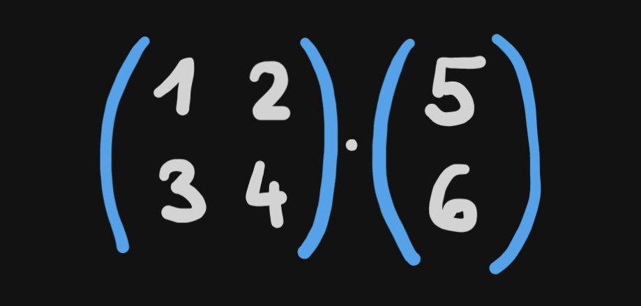
For example, the multiplication below:
can be drawn as a point going from x=10 y=0 (*) to x=26 y=-11 (**). In turn, the 2 by 2 matrix can be thought of as a set of instructions on how to move the point.
Now imagine that you’re not looking at a single point, you’re looking at a whole bunch of points all being transformed by the same matrix. What would you see? This is what Gould shows in the fifth figure of the blog post, and it’s what inspired me to create this demo in bokeh. Take a look!
Note
Clicking the image will open the demo.
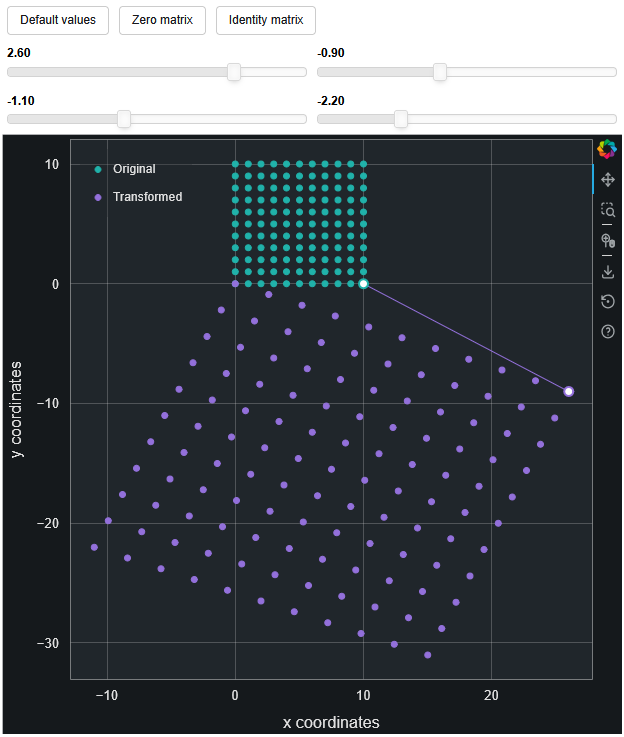
- The green points represent the original
xandycoordinates before being transformed by the 2 by 2 matrix. - The purple points represent the
xandycoordinates after being transformed by the 2 by 2 matrix. - Using the default settings, the purple line connecting the green (*) and purple point (**) depicts the transformation in the matrix multiplication example earlier.
The added benefit of this interactive approach is that you can try out different values in the 2 by 2 matrix to see what happens. I like to imagine the purple field of points as some kind of a stretchy piece of paper, where each slider (i.e., each element of the 2 by 2 matrix) stretches the paper in a different direction, with 2 corners of the paper always pinned down. In addition, the bottom-row sliders appear to warp the paper up and down while the top-row sliders stretch it left and right.
In fact, a similar space-bending effect can be seen in 3Blue1Brown’s videos on linear algebra4 5 or part of ChanRT’s Visualize It project on GitHub.6 By illustrating this transformation using grid lines, 3Blue1Brown stresses that the key property of this act of “smooshing around space” is that the grid lines are spaced out evenly and stay parallel even after the transformation takes place.
As a visual learner, I found this approach quite helpful in better understanding the intuition behind matrix multiplication. I hope it’s been beneficial to you as well. For those of you interested in how this relates to linear regression, consider finishing Gould’s original post on the Stata blog.7
Source code
Want to generate your own version of the demo? Here’s how:
- Install
uvhttps://docs.astral.sh/uv/#installation - Copy the script below to a file named, for example,
myscript.py - Open up a your terminal where you saved the script and type:
uv run myscript.py
Footnotes
Gould, W. (2011). Understanding matrices intuitively, part 1. Stata blog. URL: https://blog.stata.com/2011/03/03/understanding-matrices-intuitively-part-1/↩︎
Gould, W. (2011). Understanding matrices intuitively, part 1. Stata blog. URL: https://blog.stata.com/2011/03/03/understanding-matrices-intuitively-part-1/↩︎
3Blue1Brown (2016). Linear transformations and matrices | Chapter 3, Essence of linear algebra. YouTube. URL: https://www.youtube.com/watch?v=kYB8IZa5AuE↩︎
3Blue1Brown (2016). Matrix multiplication as composition | Chapter 4, Essence of linear algebra. YouTube. URL: https://www.youtube.com/watch?v=XkY2DOUCWMU↩︎
ChanRT. Visualize It. GitHub. URL: https://visualize-it.github.io/linear_transformations/simulation.html↩︎
Gould, W. (2011). Understanding matrices intuitively, part 1. Stata blog. URL: https://blog.stata.com/2011/03/03/understanding-matrices-intuitively-part-1/↩︎
Reuse
Content of this blogpost is licensed under Creative Commons Attribution CC BY 4.0. Any content used from other sources is indicated and is not covered by this license.
(View License)